I have picked up the Numerical Optimization book by Nocedal and Wright today. I just wanted to spend some time revisiting this topic and if I manage to stick to it for a while, maybe implement a couple of algorithms myself as a fun project.
The mathematical optimization problem
\[\begin{aligned} \min_{x \in \mathbb{R}^n} & \quad f(x) \\ \text{subject to} & \quad c_i(x) = 0, \quad i \in \mathcal{E} \\ & \quad c_i(x) = 0, \quad i \in \mathcal{I} \end{aligned}\]Here, \(x\) is a vector of decision variables, \(f\) is an objective function that we want to minimize and \(c_i\) are the constraints that the decision variables must satisfy. \(\mathcal{E}\) and \(\mathcal{I}\) are sets of indices for equality and inequality constraints respectively.
For some problems, the decision variables are all required to be integers, or binary values. In this case we call this an integer programming problem. If some of the decision variables are NOT restricted to be integers or binary values, the problem is called a mixed integer programming (MIP). Integer programming, MIPs and problems where decision variables are to be picked as permutations of an ordered set, all fall under the category of discrete optimization problems. The decision variables in this case are to be searched within a finite set. Continuous optimization problems search for decision variables in a continuous search space, i.e. \(x_i\) are real numbers.
When the objective function and the constraints are all linear functions of \(x\), the problem is called a linear programming problem. If at least some of the constraints or the objective function are nonlinear functions, the problem becomes a nonlinear programming problem.
Global optimization aims to identify the lowest function value among ALL of the feasible points. Local optimization aims to identify the lowest function value in a particular region of the feasible set.
Convexity
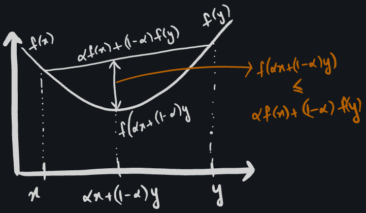
A set \(S \in \mathbb{R}^n\) is called a convex set if the straight line connecting two points in the set lies entirely within the set. To put it mathematically, if \(x \in S\) and \(y \in S\), any point on the line connecting these points can be parametrized using \(\alpha \in [0, 1]\) (lerp?). \(S\) is a convex set if \(\alpha x + (1 - \alpha y) \in S\). A function \(f\) is a convex function if its domain \(S\) is a convex set and for any two points \(x\) and \(y\) in \(S\),
\[f(\alpha x + (1 - \alpha y)) \leq \alpha f(x) + (1 - \alpha)f(y), \quad \text{for all} \quad \alpha \in [0, 1]\]
Convex programming is a special case of constrained optimization problem where the objective is convex, the equality constraint functions are linear and inequality constraint function are concave (why concave?).
I aim to write small posts like this to summarize my learnings. In the next post, I’ll share important learnings from Chapter 2 of the book: Fundamentals of Unconstrained Optimization.
